Model 2 - Tutorial 2 - Automatic detection of COVID-19 cases from chest X-ray images

Main objective of the project: Automate the process of detecting COVID-19 cases from chest radiograph images, using convolutional neural networks (CNN) through deep learning techniques. The complete project can be accessed here

Steps to reach the goal:
1- Data pre-processing
2- Model training and exposure of results

Step 2 - Model training and exposure of results

Databases used:

• X-ray images and chest CT scans of individuals infected with COVID-19 (COHE; MORRISON; DAO, 2020): link
  
• Images of lungs of individuals without any infection (KERMANY; ZHANG; GOLDBAUM, 2018): link
  

Packages used:

• Pandas
  
• Os
  
• PIL
  
• Tensorflow
  
• Sklearn
  
• Imutils
  
• Matplotlib
  
• Numpy
  
• Argparse
  
• Cv2
  
• Seaborn
  

Code used in the project:
The notebook with all the codes used in this step is available here
Note: the numbering and title of each step described in this tutorial correspond with the numbering and title contained in the notebook.

Steps to be followed:
1º Step – Import the libraries to be used
2º Step – Load the arrays built in the data pre-processing step and normalize the input data
3º Step – Split data into training data and test data
4º Step – Determining the architecture of the model (Xception) to be trained
5º Step – Determine the hyperparameters and compile the model (Xception)
6º Step – Train the model (Xception)
7º Step – Observe the accuracy of the model (Xception) and the loss function
8º Step – Determining the architecture of the model (ResNet50V2) to be trained
9º Step – Determine the hyperparameters and compile the model (ResNet50V2))
10º Step - Train the model (ResNet50V2))
11º Step - Observe the accuracy of the model (ResNet50V2) and the loss function
12º Step - Determining the architecture of the model (VGG-16) to be trained
13º Step - Determine the hyperparameters and compile the model (VGG-16)
14º Step - Train the model (VGG-16)
15º Step - Observe the accuracy of the model (VGG-16) and the loss function
16º Step - Observe which images the model (VGG16) got correctly

Tutorial 2:

1º Step

Import the libraries to be used

We import the Tensorflow, Sklearn, Imutils, Matplotlib, Numpy, Argparse, Cv2, Os, Pandas and Seaborn libraries, since we will rely on them to carry out the training of the model referring to COVID-19 and the analysis of the results.

from tensorflow.keras.preprocessing.image import ImageDataGenerator
from tensorflow.keras.applications import VGG16
from tensorflow.keras.applications import Xception
from tensorflow.keras.applications import ResNet50V2
from tensorflow.keras.layers import AveragePooling2D
from tensorflow.keras.layers import MaxPooling2D
from tensorflow.keras.layers import Dropout
from tensorflow.keras.layers import Flatten
from tensorflow.keras.layers import Conv2D
from tensorflow.keras.layers import Dense
from tensorflow.keras.callbacks import ReduceLROnPlateau
from tensorflow.keras.layers import Input
from tensorflow.keras.models import Model
from tensorflow.keras.optimizers import Adam
from tensorflow.keras.utils import to_categorical
from sklearn.preprocessing import LabelBinarizer
from sklearn.model_selection import train_test_split
from sklearn.metrics import classification_report
from sklearn.metrics import confusion_matrix
from imutils import paths
import matplotlib.pyplot as plt
import numpy as np
import argparse
import cv2
import os
from sklearn.model_selection import train_test_split
from sklearn.metrics import confusion_matrix
import pandas as pd
import seaborn as sn
%matplotlib inline

Note: some libraries have not been imported completely, such as, for example, Tensorflow, as we will not use all the functions contained therein. In this way, it facilitates the use of the library and the processing of codes/data.

2º Step

Load the arrays built in the data pre-processing step and normalize the input data

The “X_Train” and “Y_Train” arrays built in Step 1 were loaded and associated, respectively, with the variables “X_train” and “Y_train”. In addition, the variable X_train has been normalized for values ​​ranging from 0 to 1.

X_train = np.load("/content/drive/My Drive/Python/COVID/Arrays/Modelo2/X_Train.npy")
X_train = X_train/255
Y_train = np.load("/content/drive/My Drive/Python/COVID/Arrays/Modelo2/Y_Train.npy")

3º Step

Split data into training data and test data

20% of the data referring to the images were separated for the model test. The function below returns four values that have been associated with four variables, namely: “X_train”, “X_test”, “Y_train” and “Y_test”.

X_train,X_test,Y_train,Y_test = train_test_split(X_train,Y_train, test_size = 0.2, random_state = 40)

Note: the “random_state” parameter makes the random selection of images the same every time the function is executed.

4º Step

Determining the architecture of the model (Xception) to be trained

The weights of the Xception architecture were loaded from the “imagenet” dataset, disregarding the top of the network. In addition, the input was defined with the size of the images in the image bank that we will use, namely: 237 x 237px and 3 color channels as depth. This information was associated with the “bModel” variable.

In addition, the architecture of the top of the network was determined, since the top of the network was removed from the “imagenet” dataset. This architecture was associated with the “tModel” variable.

Finally, the “bModel” and “tModel” variables were merged into the “model” variable. This last variable represents the model that will be trained.

bModel = Xception(weights="imagenet", include_top=False,
  	input_tensor=Input(shape=(237, 237, 3)))
tModel = bModel.output
tModel = AveragePooling2D(pool_size=(2, 2))(tModel)
tModel = Flatten(name="flatten")(tModel)
tModel = Dense(20, activation="relu")(tModel)
tModel = Dropout(0.2)(tModel)
tModel = Dense(3, activation="softmax")(tModel)

model = Model(inputs=bModel.input, outputs=tModel)

5º Step

Determine the hyperparameters and compile the model (Xception)

The hyperparameters, in particular, the learning rate (“INIT_LR”), the epochs (“EPOCHS”) and the batch size (“BS”) were determined.

Subsequently, the Adam optimization function (“opt”) was defined, the model was compiled considering the loss function “categorical_crossentropy” and as a metric for evaluating the results, accuracy was considered.

INIT_LR = 1e-3
EPOCHS = 80
BS = 15

for layer in bModel.layers:
    layer.trainable = False

opt = Adam(lr=INIT_LR)
model.compile(loss="categorical_crossentropy", optimizer=opt,
    metrics=["accuracy"])

6º Step

Train the model (Xception)

From the command below, the model was trained, leaving 10% of the images for validation. The information was saved in variable “x” and the model was saved on the computer as “modeloc_2.hdf5”.

reduce_lr = ReduceLROnPlateau(monitor='val_loss', factor=0.2,
                              patience=5, min_lr=0.001, cooldown=5)

x = model.fit(X_train, Y_train, batch_size=BS,validation_split=0.1, epochs=EPOCHS,callbacks=[reduce_lr])

model.save("/content/drive/My Drive/Python/COVID/model/modeloc_2.hdf5")

7º Step

Observe the accuracy of the model (Xception) and the loss function

We built a graph to analyze the accuracy history of training data and model validation. We also built a graph that computes the network error in relation to the training and validation data. They point out that, apparently, there was no overfitting, since the training and validation lines approached.

In addition, it is noted that the model’s accuracy was 94%. That is, the model hit 94% of the images used in the test.

plt.plot(x.history['accuracy'])
plt.plot(x.history['val_accuracy'])
plt.title('model accuracy')
plt.ylabel('accuracy')
plt.xlabel('epoch')
plt.legend(['train', 'validation'], loc='upper left')
plt.show()

plt.plot(x.history['loss'])
plt.plot(x.history['val_loss'])
plt.title('model loss')
plt.ylabel('loss')
plt.xlabel('epoch')
plt.legend(['train', 'validation'], loc='upper left')
plt.show()

model.evaluate(X_test,Y_test)

3/3 [==============================] - 1s 396ms/step - loss: 0.2876 - accuracy: 0.9467
[0.287587970495224, 0.9466666579246521]

8º Step

Determining the architecture of the model (ResNet50V2) to be trained

The weights of the ResNet50V2 architecture were loaded from the “imagenet” dataset, disregarding the top of the network. In addition, the input was defined with the size of the images in the image bank that we will use, namely: 237 x 237px and 3 color channels as depth. This information was associated with the “bModel” variable.

In addition, the architecture of the top of the network was determined, since the top of the network was removed from the “imagenet” dataset. This architecture was associated with the “tModel” variable.

Finally, the “bModel” and “tModel” variables were merged into the “model” variable. This last variable represents the model that will be trained.

bModel = ResNet50V2(weights="imagenet", include_top=False,
  	input_tensor=Input(shape=(237, 237, 3)))
tModel = bModel.output
tModel = AveragePooling2D(pool_size=(2, 2))(tModel)
tModel = Flatten(name="flatten")(tModel)
tModel = Dense(20, activation="relu")(tModel)
tModel = Dropout(0.2)(tModel)
tModel = Dense(3, activation="softmax")(tModel)

model = Model(inputs=bModel.input, outputs=tModel)

9º Step

Determine the hyperparameters and compile the model (ResNet50V2)

The hyperparameters, in particular, the learning rate (“INIT_LR”), the epochs (“EPOCHS”) and the batch size (“BS”) were determined.

Subsequently, the Adam optimization function (“opt”) was defined, the model was compiled considering the loss function “categorical_crossentropy” and as a metric for evaluating the results, accuracy was considered.

INIT_LR = 1e-3
EPOCHS = 80
BS = 15

for layer in bModel.layers:
    layer.trainable = False

opt = Adam(lr=INIT_LR)
model.compile(loss="categorical_crossentropy", optimizer=opt,
    metrics=["accuracy"])

10º Step

Train the model (ResNet50V2)

From the command below, the model was trained, leaving 10% of the images for validation. The information was saved in variable “x” and the model was saved on the computer as “modeloc_2.hdf5”.

reduce_lr = ReduceLROnPlateau(monitor='val_loss', factor=0.2,
                              patience=5, min_lr=0.001, cooldown=5)

x = model.fit(X_train, Y_train, batch_size=BS,validation_split=0.1, epochs=EPOCHS,callbacks=[reduce_lr])

model.save("/content/drive/My Drive/Python/COVID/model/modeloc_2.hdf5")

11º Step

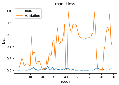
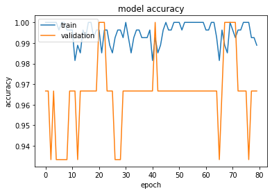
Observe the accuracy of the model (ResNet50V2) and the loss function

We built a graph to analyze the accuracy history of training data and model validation. We also built a graph that computes the network error in relation to the training and validation data. They point out that, apparently, there was no overfitting, since the training and validation lines approached.

In addition, it is noted that the model’s accuracy was 96%. That is, the model hit 96% of the images used in the test.

plt.plot(x.history['accuracy'])
plt.plot(x.history['val_accuracy'])
plt.title('model accuracy')
plt.ylabel('accuracy')
plt.xlabel('epoch')
plt.legend(['train', 'validation'], loc='upper left')
plt.show()

plt.plot(x.history['loss'])
plt.plot(x.history['val_loss'])
plt.title('model loss')
plt.ylabel('loss')
plt.xlabel('epoch')
plt.legend(['train', 'validation'], loc='upper left')
plt.show()

model.evaluate(X_test,Y_test)

3/3 [==============================] - 1s 346ms/step - loss: 0.3698 - accuracy: 0.9600
[0.3697645366191864, 0.9599999785423279]

12º Step

Determining the architecture of the model (VGG-16) to be trained

The weights of the VGG-16 architecture were loaded from the “imagenet” dataset, disregarding the top of the network. In addition, the input was defined with the size of the images in the image bank that we will use, namely: 237 x 237px and 3 color channels as depth. This information was associated with the “bModel” variable.

In addition, the architecture of the top of the network was determined, since the top of the network was removed from the “imagenet” dataset. This architecture was associated with the “tModel” variable.

Finally, the “bModel” and “tModel” variables were merged into the “model” variable. This last variable represents the model that will be trained.

bModel = VGG16(weights="imagenet", include_top=False,classes=3,
	input_tensor=Input(shape=(237, 237, 3)))
  tModel = bModel.output
tModel = AveragePooling2D(pool_size=(2, 2))(tModel)
tModel = Flatten(name="flatten")(tModel)
tModel = Dense(20, activation="relu")(tModel)
tModel = Dropout(0.2)(tModel)
tModel = Dense(3, activation="softmax")(tModel)

model = Model(inputs=bModel.input, outputs=tModel)

13º Step

Determine the hyperparameters and compile the model (VGG-16)

The hyperparameters, in particular, the learning rate (“INIT_LR”), the epochs (“EPOCHS”) and the batch size (“BS”) were determined.

Subsequently, the Adam optimization function (“opt”) was defined, the model was compiled considering the loss function “categorical_crossentropy” and as a metric for evaluating the results, accuracy was considered.

INIT_LR = 1e-3
EPOCHS = 80
BS = 15

for layer in bModel.layers:
    layer.trainable = False

opt = Adam(lr=INIT_LR)
model.compile(loss="categorical_crossentropy", optimizer=opt,
    metrics=["accuracy"])

14º Step

Train the model (VGG-16)

From the command below, the model was trained, leaving 10% of the images for validation. The information was saved in variable “x” and the model was saved on the computer as “modeloc_2.hdf5”.

reduce_lr = ReduceLROnPlateau(monitor='val_loss', factor=0.2,
                              patience=5, min_lr=0.001, cooldown=5)

x = model.fit(X_train, Y_train, batch_size=BS,validation_split=0.1, epochs=EPOCHS,callbacks=[reduce_lr])

model.save("/content/drive/My Drive/Python/COVID/model/modeloc_2.hdf5")

15º Step

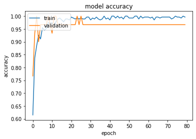
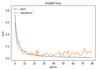
Observe the accuracy of the model (VGG-16) and the loss function

We built a graph to analyze the accuracy history of training data and model validation. We also built a graph that computes the network error in relation to the training and validation data. They point out that, apparently, there was no overfitting, since the training and validation lines approached.

In addition, it is noted that the model’s accuracy was 97%. That is, the model hit 97% of the images used in the test.

plt.plot(x.history['accuracy'])
plt.plot(x.history['val_accuracy'])
plt.title('model accuracy')
plt.ylabel('accuracy')
plt.xlabel('epoch')
plt.legend(['train', 'validation'], loc='upper left')
plt.show()

plt.plot(x.history['loss'])
plt.plot(x.history['val_loss'])
plt.title('model loss')
plt.ylabel('loss')
plt.xlabel('epoch')
plt.legend(['train', 'validation'], loc='upper left')
plt.show()

model.evaluate(X_test,Y_test)

3/3 [==============================] - 1s 177ms/step - loss: 0.0941 - accuracy: 0.9733
[0.09413935989141464, 0.9733333587646484]

16º Step

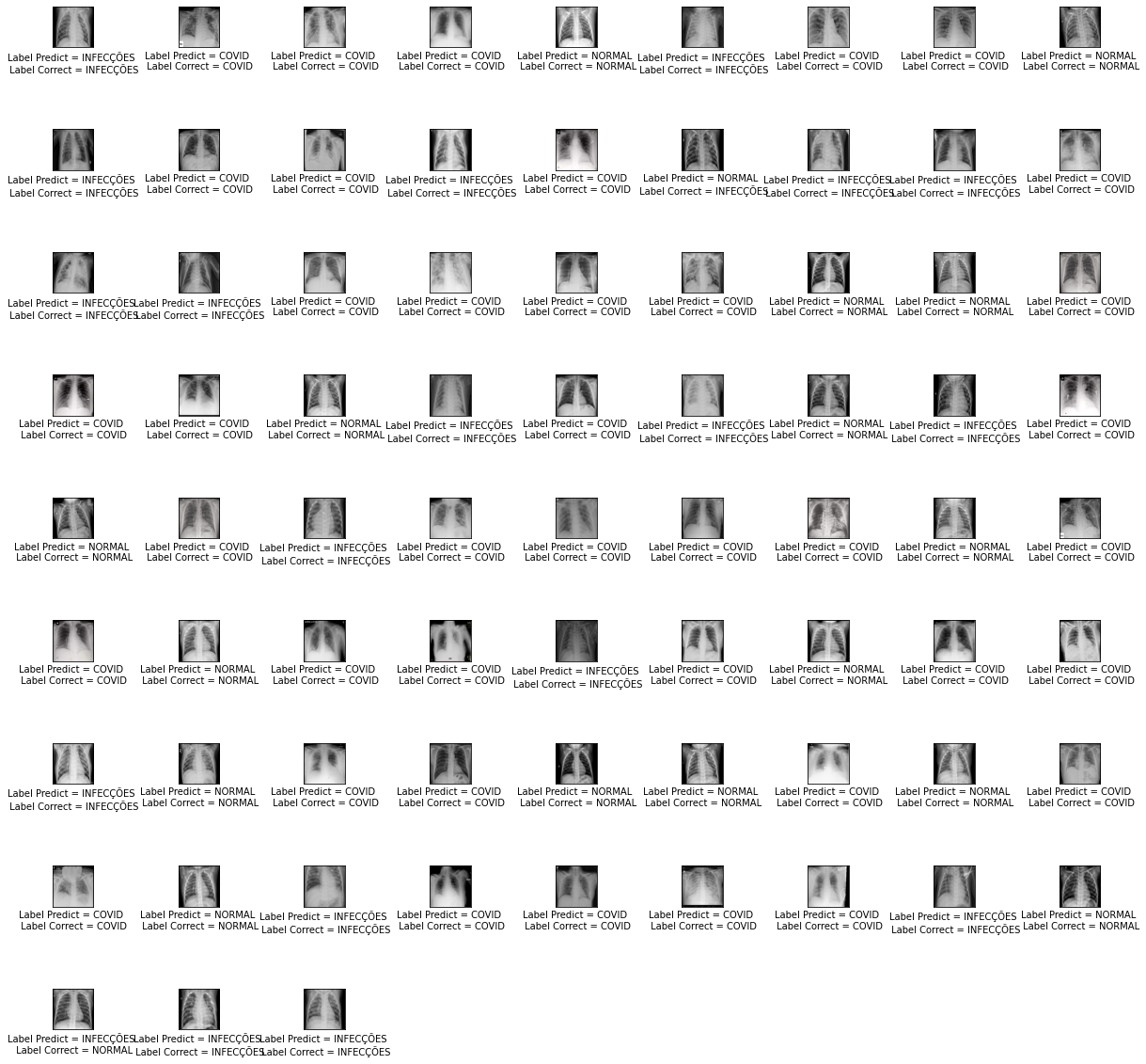
Observe which images the model (VGG16) got correctly

From the image below it is possible to see the images that the model got right. The “Labels” (Label Predict and Label Correct) that have the same name indicate that the model has correctly predicted. Example: Label Predict = COVID and Label Correct = COVID.

In addition, the figure was saved as modelo_2.pdf on the computer.

plt.figure(figsize=(20,20))
plt.subplots_adjust(left=None, bottom=None, right=None, top=None, wspace=2.0, hspace=2.0)
i = 0
for i,image in enumerate(X_test):
    plt.subplot(9,9,i+1)
    plt.xticks([])
    plt.yticks([])
    plt.grid(False)
    plt.imshow(image, cmap=plt.cm.binary)
    img = np.expand_dims(X_test[i],axis = 0)
    x_pred = model.predict(img)[0]
    pred_covid = x_pred[0]
   
    pred_normal = x_pred[1]

    pred_infeccoes = x_pred[2]
    
    
    if pred_covid > pred_normal and pred_covid > pred_infeccoes:
      label = "COVID"
    elif pred_normal > pred_covid and pred_normal > pred_infeccoes:
      label = "NORMAL"
    elif pred_infeccoes > pred_covid and pred_infeccoes > pred_normal:
      label = "INFECÇÕES"
     
    
    if Y_test[i][0] == 1:
      label_test = "COVID"
    elif Y_test[i][1] == 1:
      label_test = "NORMAL"
    elif Y_test[i][2] == 1:
      label_test = "INFECÇÕES"
    plt.xlabel(f"Label Predict = {label} \n Label Correct = {label_test}")
    i += 1
plt.savefig('/content/drive/My Drive/Python/COVID/model/modelo_2.pdf')

Conclusion on model 2: From the preliminary results, it is possible to notice that the model has a high accuracy to classify the normal lungs, with COVID-19, and other infections. Especially from the VGG-16 architecture. The next training session will test new architectures and parameters in order to improve the model.


Note: the results are not clinical, but exploratory. However, with the improvement of the models, they can bring benefits to confront COVID-19.

Bibliography
COHEN, Joseph; MORRISON, Paul; DAO, Lan. COVID-19 Image Data Collection. arXiv:2003.11597, 2020.

KERMANY, Daniel; ZHANG, Kang; GOLDBAUM, Michael. Labeled Optical Coherence Tomography (OCT) and Chest X-Ray Images for Classification. Mendeley Data, v.2, 2018. Disponível em: http://dx.doi.org/10.17632/rscbjbr9sj.2